2. ABOUT THE CROP GROWTH MONITORING SYSTEM
2.1. Introduction
The JRC (i.e. European Commission) requested Alterra (formerly SC-DLO) and Plant Research International (formerly AB-DLO) in Wageningen, The Netherlands, to develop, adapt and calibrate new or existing agro-meteorological simulation models for:
- 10-day routine quantitative forecasting of national and regional yields (per unit area).
- Qualitative monitoring of the growth conditions for the whole EU for the following crops: wheat (spring, winter, soft and durum), oats, grain maize, rice, potato, sugar beet, pulses, soybean, oilseed rape, sunflower, tobacco and cotton. (Olives and grapes were covered by another subproject).
Figure 2.1. presents a schematic overview of CGMS; three levels can be distinguished. The first level is the weather system. Historical and actual weather data are collected, corrected and subsequently interpolated to the grid centre. The CGMS system as used by the European Commission is based on a 50 x 50 km grid. Other CGMS systems may use a different grid size. Historical, actual and interpolated meteorological data are stored in a database. The interpolated data are subsequently introduced in WOFOST. Figure 2.2. presents a schematic overview of the weather system (Level 1). At the second level, crop growth simulation takes place (Figure 2.3.). In addition to the interpolated data obtained at Level 1, crop characteristics and soil information are needed as input for WOFOST.
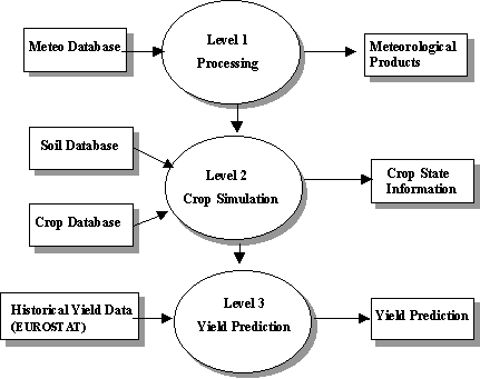
Figure 2.1. Schematic overview of the Crop Growth Monitoring System.
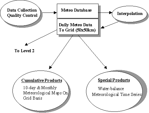
Figure 2.2. Schematic overview of Level 1
In Subsections 2.2.3. and 2.2.4. the crop and soil databases linked to CGMS are described. Simulations are performed per Elementary Mapping Unit (EMU), which is the intersection of a Soil Mapping Unit (SMU, see Subsection 2.2.4.), a grid cell and an administrative region. The administrative regions used in the current operational version of CGMS at the JRC are called Nomenclatures des Unités Territoriales Statistiques (NUTS). Simulation results may subsequently be aggregated to subregional, regional and national level, e.g. from NUTS2 to NUTS1 and finally to NUTS0 (see Section 2.4.). In the current operational version of CGMS, simulation results are aggregated to national level (NUTS0) and the national yield per unit area is predicted (Level 3, see Figure 2.4.).
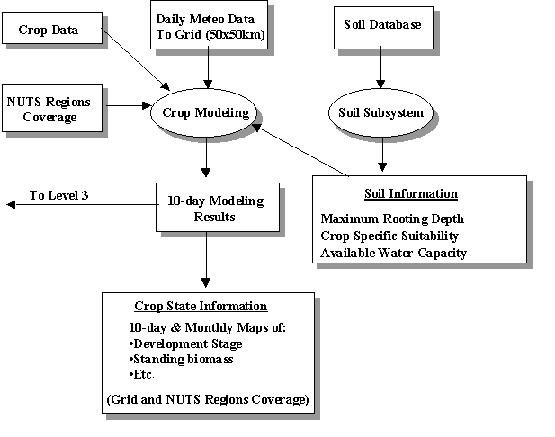
Figure 2.3. Schematic overview of Level 2
Various simulation results are regressed on historical yield observations. The simulation result yielding the highest coefficient of determination is selected as predictor and subsequently introduced in the prediction routine. In Section 2.6. the prediction model and the applied prediction method are described, respectively. Yield and production volume prediction are performed every 10 days. (see Section 2.7.).
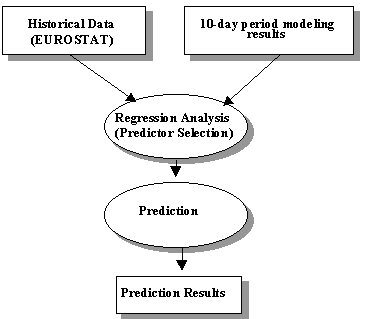
Figure 2.4. Schematic overview of the prediction system (Level
3)
2.2. Data and databases
One of the goals of the MARS project was to develop an operational
system to forecast production volumes of various crops at European Union
level. For this system development, it was essential to identify
useful parameters that are measured across Europe and to check whether
they are available at such a resolution that they could be used for regional
crop growth modeling. For static variables, such as soil characteristics
and long-term mean meteorological variables, existing data had to be inventoried
to assess the possibility to compile and harmonize this information across
the EU. For dynamic parameters, such as daily weather variables, data had
to be limited to those that were regularly collected and could be received
and processed in semi real time.
Based on these criteria an initial set of available input data was defined,
consisting of historical daily meteorological data from approximately 380
stations, current season daily weather data from about 700 stations, topography
at a 5 minute grid, regional crop parameters, historical crop statistics
per administrative unit and the EU soil data base at a scale of 1,000,000.
Compilation of the identified parameters and development of the MARS databases
proceeded in parallel with the development of CGMS. An overview of the CGMS
database and its tables is presented in
Appendix V.
2.2.1. Meteorological data
The meteorological data used at the JRC for Level 1 are collected from the Global Telecommunication System (GTS) of the World Meteorological Organisation (WMO). The meteorological database contains information on the meteorological stations, daily meteorological data and interpolated data, respectively. The station information stored is WMO number, station name, longitude, latitude and altitude. Furthermore, it contains the meteorological observations obtained via GTS, comprising 29 different parameters, including various indicators for cloud cover, temperature and vapor pressure. Unfortunately, many stations across Europe measure only limited subsets of these parameters. Meteorological data used as input in CGMS are: minimum and maximum temperature, rainfall, windspeed, vapor pressure and global radiation or sunshine duration. Only stations that report at least this set of variables on a daily basis are included in the database. Daily potential evapotranspiration is calculated from these data and is also included in the database.
The subproject to compile historical meteorological data stretched over a period of 5 years. The historical datasets (1949-1991) were ordered directly from the national meteorological services. Data from all EU member states and from Poland and Slovenia were acquired, converted to consistent units and scanned for inconsistencies (e.g. minimum temperature higher than maximum temperature).
In 1992, daily meteorological data were received from approximately 750 stations. In 1998 this number had increased to over 1200. Figure 2.5. presents part of the network of meteorological stations included in the meteorological database.
Meteorological data are preprocessed using the AMDAC software package (Meteo-Consult, 1991), which decodes the incoming data and checks their consistency. Individual meteorological parameters are compared to those of surrounding stations and to other observations that are obtained on the same day for the same station. Obvious errors in the observations are corrected automatically, possible errors are marked for manual correction later on and a message is written to a log file.
Figure 2.5. Network of meteorological stations that broadcast data via GTS and whose data are stored in the meteorological database.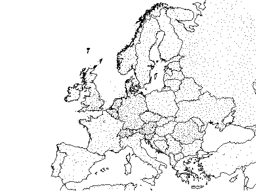
Missing values are replaced through temporal and spatial interpolation, provided sufficient "surrounding" information is available, otherwise they remain blank.
Meteorological input for CGMS is based on a
grid, which dimensions
depend on the implementation (the EC uses a 50 x 50km grid, other implementations
apply 20 x 20km or 10 x 10km). A methodology
for data interpolation from the existing network of meteorological stations
to the grid center was developed on the basis of the studies of Beek et
al. (1992) and van der Voet et al. (1993). The interpolation
procedure selects an optimum set of stations and an average value of observed
data is attributed to the grid center, without weighting for distance.
Rainfall is taken from the nearest station. Selection of the optimum set
of stations is based on the following criteria: proximity to other stations,
similarity in altitude and distance to the coast, position in relation
to climatic barriers (i.e. mountain ranges) and a regular configuration
surrounding the grid center. An overview of the tables containing the
meteorological data is presented in
Appendix VI
2.2.2. Crop characteristics database and crop knowledge base
Data describing the specific growth potentials of individual crops are an essential input to any crop growth simulation model. A subproject was launched to collect and compile all data that could possibly be transformed to either crop characteristics, used as input in CGMS, or information to be included in the crop knowledge base. This knowledge base provides information on (i) meteorological and other types of hazards likely to affect crop yield, (ii) crop requirements with respect to soil characteristics, climatic zones, etc. The collected data can be divided in the following categories:
- Basic non-region specific crop physiological data such as rooting depth, temperature threshold for growth, etc. This information was derived from literature.
- Agronomic data such as: varieties grown in a region and the earliest and latest dates of sowing and harvest for these varieties; maximum altitude at which a crop is grown, etc.
- Detailed physiological information such as heat sums to reach various phenological stages, energy conversion, partitioning of assimilates over various plant organs, etc. This information was derived from literature. For wheat, information was also derived from field trials executed in Belgium, United Kingdom and the Netherlands. For other countries, no detailed field observations were available and consequently calibration of the crop characteristics could not be executed (Boons-Prins et al., 1993).
Results of this subproject are presented by Russell & Wilson
(1994), Carbonneau et al. (1992), Falisse (1992), Narisco et
al. (1992), Bignon (1990), Falisse & Decelle, (1990), Hough (1990)
and Russell (1990). Boons-Prins et al. (1993) used these results
and constructed crop files used as input in CGMS, including also information
from van Heemst (1988) and van Diepen & de Koning (1990).
Crop files have been constructed for: winter wheat, spring wheat, barley,
rice, potato, sugar beet, field beans, soybean, oilseed rape and sunflower.
For some crops, crop files for specific varieties grown in certain regions
have been constructed. In addition, each crop is assigned to one of the
following crop groups: grasses, cereals and root crops. Requirements of
these crop groups with respect to soil-related characteristics such as
phase, texture, alkalinity, salinity, etc. are stored in the crop database.
An overview of the tables containing the crop characteristics
is presented in Appendix VII
2.2.3. European soil and geographical database
The JRC applies the 1:1.000.000 INRA soil map, in combination with the 1:5.000.000 FAO soil map. A 1:250.000 soil map is being used in other, smaller installations. The scale of the soil map has a direct impact on the number of Elementary Mapping Units (EMU), and therefore a direct impact on the system size and the processing time required. In Heineke et al. (1998), a detailed description of present situation is presented. The soil database consists of four parts:
- The meta-database, containing information on the soil surveys executed in Europe. It provides a catalogue with information on national maps and datasets.
- The geographical database, containing the list of Soil Typological Units (STU), i.e. all soil types within the EU identified on the basis of the FAO-UNESCO (1974) legend. The STUs are described by soil attributes with a harmonized coding, such as: FAO soil name, parent material, slope, etc. STUs are generally too small to be distinguished on a map at scale 1:1,000,000. Therefore, they are clustered in Soil Mapping Units (SMU). The concept of SMU is related to that of soil associations postulated by Simonson (1971).
- The soil profile analytical database, containing soil profile descriptions, including results of physical and chemical analyses (Madsen & Jones, 1996). Data are stored in two categories, the first containing the measured data from georeferenced profiles, the second contains estimated data. About 300 profiles are currently available, representing the most important STUs.
- The knowledge database, containing the pedotransfer rules, i.e. simple deductive functions to derive soil parameters from available data (King et al., 1994b) and to formalize empirical interpretation when using soil maps (Jones & Hollis, 1996; Van Ranst et al., 1995)
2.2.4. Historical yield and planted area data
Statistics on planted area, yield and production volume as applied at
Level 3 (see Figure 2.4.) have been collected from
national statistical services of all EU member states by EUROSTAT. Within
the EU, no single Community system to establish these statistics exists:
the methods applied vary from country to country. Through article 3 of
CAP regulation 837/90, the Commission attempts to harmonize these methods
and to stimulate the use of scientific procedures. This regulation prescribes
amongst others that censuses or representative sample surveys shall obtain
data on planted area, yield and production volume for all significant crops.
Bradbury (1994) investigated the applied methods to establish these statistics
for cereals for various EU member states. He concluded that "most member
states attempt to estimate sampling errors, and usually manage to show
that the margins are close enough to those set out in regulation 837/90,
but with greater or lesser amount of convincing detail. For judgmental
assessment of yield (and for Greece, of area as well) no fully satisfactory
methods to establish the estimating error are available, for the simple
reason that it is not a scientific method."
2.3. The applied crop growth simulation model
The heart of CGMS, used for the Level 2 crop simulation, is the WOFOST crop growth simulation model, whose underlying principles have been discussed by van Keulen & Wolf (1986). The initial version of this model was developed by the Centre for World Food Studies and AB-DLO (van Diepen et al., 1989; 1988). Implementation in CGMS and its structure is described by Supit et al. (1994). Technical descriptions and user manuals have been prepared by van Raaij & van der Wal (1994), van der Wal, (1994) and Hooijer et al. (1993).
WOFOST calculates first the instantaneous photosynthesis at three depths in the canopy for three moments of the day, which is subsequently integrated over the depth of the canopy and over the light period, to arrive at daily total canopy photosynthesis. After subtracting maintenance respiration, assimilates are partitioned over roots, stems, leaves and grains as a function of the development stage, which is calculated by integrating the daily development rate, described as a function of temperature and photoperiod. Assimilates are then converted into structural plant material taking into account growth respiration. Growth is driven by temperature and limited by assimilate availability. Figure 2.6. presents a schematic overview of these processes.
Aboveground dry matter accumulation and its distribution over leaves, stems and grains on a hectare basis are simulated from sowing to maturity on the basis of physiological processes as determined by the crop. s response to daily weather (rainfall, solar radiation, photoperiod, minimum and maximum temperature and air humidity), soil moisture status (i.e. Ta/Tp in Figure 2.6.) and management practices (i.e. sowing density, planting date, etc.). Water supply to the roots, infiltration, runoff, percolation and redistribution of water in a one-dimensional profile are derived from hydraulic characteristics and moisture storage capacity of the soil.
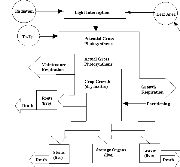
Figure 2.6. Crop growth processes simulated by WOFOST. Taand Tp are actual and potential transpiration rate (de Koning et al., 1993).
The required inputs per grid cell are daily weather data, soil characteristics and management practices (i.e. sowing density, planting date, etc.). Daily weather data are obtained from the GTS and interpolated to the grid-center (see Section 2.2.).
CGMS simulates two production situations: potential and water-limited. The potential situation is defined by temperature, daylength, solar radiation and crop characteristics (e.g. leaf area dynamics, assimilation characteristics, dry matter partitioning, etc.). The water-limited situation is characterized by the aforementioned factors plus: water availability derived from root characteristics, soil physical properties, rainfall and evapotranspiration. In both situations, optimal supply of nutrients is assumed and for each situation, total aboveground dry matter and grain dry matter per hectare are calculated.
As input for the prediction models the following simulation results
may be used: potential grain yield, water-limited grain yield, potential
aboveground biomass and water-limited aboveground biomass. One of these
variables is selected as predictor. The selection procedure and prediction
method are described in Subsection 2.5.2.
2.4. Aggregation as applied by the JRC
Simulations are performed per Elementary Mapping Unit (EMU), the intersection of a Soil Mapping Unit (SMU), grid cell and administrative region. Figure 2.7. presents a schematic outline of an EMU (JRC installation). SMUs are derived from the Soil Map of the European Communities, scale 1:1,000,000. The NUTS system is organized as follows: the highest level, the whole country, is called NUTS-0, which is divided in regions: NUTS-1. Regions are subdivided in NUTS-2 subregions. In order to be able to correlate the simulation results with actual observed data, EMU simulation results are aggregated to NUTS-2 yields via:
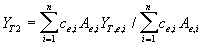
| where | e | : | EMU | [-] |
| YT2 | : | simulated average NUTS-2 yield in year T | [ton.ha-1] | |
| YT,e,i | : | simulated EMU yield in year T | [ton.ha-1] | |
| Ae | : | EMU area | [ha] | |
| ce | : | percentage of the EMU area suitable for cultivation of crop x | [-] | |
| n | : | number of EMUs in a NUTS-2 subregionof the EMU area suitable for wheat cultivation | [-] |
No information on land use at EMU level is available, therefore ce is used. This value is derived from the Soil Typological Unit (STU) table that describes soil characteristics of a SMU such as slope, texture, etc., (King et al., 1994a, b) and is invariable in time. Yield statistics at NUTS2 level are rarely available, therefore NUTS-2 yields in year T are aggregated to NUTS-1 yield via:
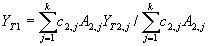
| where | 2 | : | stands for NUTS-2 | [-] |
| A2 | : | NUTS-2 area | [ha] | |
| c2 | : | c2 is percentage of the NUTS-2 area suitable for cultivation of crop x | [-] | |
| k | : | number of NUTS-2 subregions per NUTS-1 region | [-] |
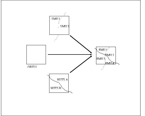
Figure 2.7. Schematic outline of the Elementary Mapping
Unit (EMU), the intersection of a Soil Mapping Unit (SMU), grid cell and
administrative region, Nomenclatures des Unités Territoriales Statistiques
(NUTS).
Simulated average NUTS-0 yield is obtained in a similar way. Although
information on actual land use at NUTS-2 level is available, in the operational
version of CGMS these data are not used for aggregation of simulation results
from NUTS-2 to NUTS-1 to NUTS-0 yield. Currently, the operational version
of CGMS aggregates simulation results to NUTS-0 level and these values
are introduced in the yield prediction routine.
For further explanation of the aggregation method see also
Appendix VIII.
2.5. Prediction model
2.5.1. The actual prediction model
Vossen (1992, 1990) proposed a combination of a linear time trend (Palm & Dagnelie, 1993; Swanson & Nyankori, 1979) and crop growth simulation results to account for the trend in yield series and weather variability, respectively. The prediction model applied in CGMS is based on this proposal. It can be described as:
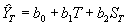
| where | : | Estimated yield in year T | [ton.ha-1] | |
| ST | : | Simulation result in year T | [ton.ha-1] | |
| b0 | : | regression constant | [ton.ha-1] | |
| b1 | : | regression constant | [ton.ha-1.year-1] | |
| b2 | : | regression constant | [-] |
The production volume ![]() (ton), in year T, can thus be estimated as:
(ton), in year T, can thus be estimated as:

| where | : | Production volume | [ton] | |
| : | Estimated planted area | [ha] |
Equation (2.3) assumes additive effects of weather on yield, i.e. yield variability as a result of weather influences, is similar under a high fertilizer input regime and under a low fertilizer input regime. Equation (2.4) assumes a linear relation between planted area and production volume, or in other words, similar yield on the total area planted. These assumptions may be challenged.
The prediction method applied in CGMS is similar to the one described
in next subsection. Historical yield values are regressed according to
equation (2.3), and the obtained regression constants are subsequently
used in the prediction model. It is assumed that these historical values
correctly represent national yields. However, each EU member state has
its own methods to establish these values and, as mentioned by Bradbury
(1994), the estimation errors are not always known. Caution should therefore
be exercised when comparing the quality of the prediction results among
the individual countries.
2.5.2. The actual prediction method
The prediction method described by Vossen & Rijks (1995) is applied. The following crop growth simulation results (on hectare basis) are examined: potential grain yield, water-limited grain yield, potential total above-ground dry matter yield and water-limited above-ground dry matter yield. For the period 1975-1994, for a moving window of 10 years, the regression coefficients are established and subsequently used for prediction of production volume or yield per hectare of the 11th year. The crop growth simulation result yielding the highest adjusted coefficient of determination over each 10-day period is used for prediction.
A smooth trend of any type over a large number of years assumes a continuity
which might be unrealistic (de Koning et al., 1993; Vossen, 1992; 1990).
The recent agricultural policy of the EU aims at a reduction of production
volume and subsidies for various crops, including wheat (Vossen & Rijks,
1995). According to these authors the predictor should only be based on
data from the recent past. The length of the series should nevertheless
be long enough to give a sufficient number of degrees of freedom in the
regression analysis. Gradual shift in the time trend is allowed for by
the shortness of the time series, used to derive the predictor.
2.6. CGMS and the MARS forecasting system
The objective of the MARS project is to predict production volumes of the major crops at national level and possibly at regional level for all EU member states. Production volume is divided in a yield and a planted area component, which are estimated separately and subsequently multiplied. Planted area is estimated using high resolution imagery and ground surveys (Scot Conseil, 1994), yield is predicted subjectively. Production volume predictions are refined in the course of the year, from an early indicator value through provisional data to final results. A panel of analysts performs these predictions on a monthly basis, form March till September. Every ten days, they also assess crop growth conditions, such as occurrences of droughts, excess rain, etc. It is assumed that changes in crop growth and development as a result of for example stress situations, can be detected by CGMS and on remote sensing images, obtained in consecutive ten-day periods. The first predictions are based on extrapolated yield and planted area time series. In the course of the season, information provided by various sources is analyzed and combined (see Figure 2.8.). Predictions and assessment are subjective and based on analysis and synthesis of:
- The rapid surface estimate system that provides estimates of the year-to-year changes in planted area of the major crops. The field surveys executed in the framework of this system provide additional information on yield and planted area.
- CGMS products produced at the Levels 1, 2 and 3 (see Figure 2.1.).
- Information on vegetation status (NDVI or surface temperature) using NOAA-AVHRR imagery processed with the SPACE/SCAN software package.
- Information from farmer magazines and experts.
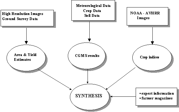
Figure 2.8. MARS yield forecasting system.
Prediction results obtained at Level 3 (i.e. the prediction model; see
Subsection
2.5.2.), indicate how crops may have reacted to weather influences.
The analysts adapt these results when, in their opinion, other factors
should be accounted for or when the predicted value is deemed to be incorrect.
For prediction, one of the following simulation results is selected: potential
yield, potential biomass, water-limited yield and water-limited biomass.
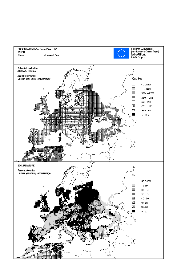
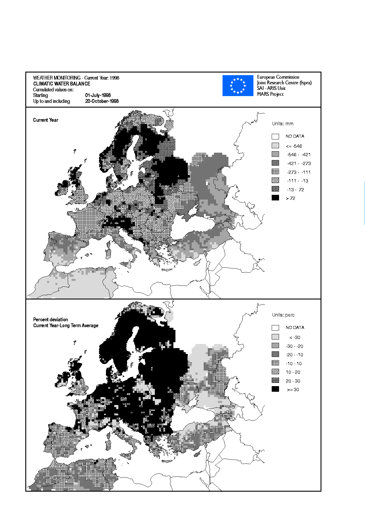
Figure 2.9. CGMS results on a 50 x 50 km grid. The upper part of this figure presents the deviation of the production per unit area at harvest time from the long-term average (i.e. the mean over 15-30 years, depending on the available data). The bottom part presents deviation of the soil moisture calculations with respect to the long-term average (i.e. the mean over 15-30 years, depending on the available data)
2.7. Omissions in CGMS
One of the processes not accounted for in CGMS is the ability of plants to adapt to low resource conditions by modifying their morphology and physiology. This capability for adjustment derives from the ability of plants to partition their assimilated energy among various morphological structures and physiological processes. Functioning of this mechanism is not clearly understood. According to Sinclair & Park (1993):"mechanistic crop models, which account for the effects of environmental variations on crop responses, have not led to a singular understanding of the resource limitations on crop yield other than a realization that a number of factors must be considered." CGMS may overestimate drought effects since this adaptive mechanism is not accounted for.
Yield reducing factors not accounted for in CGMS are amongst others: water-logging, erosion, frost. In addition, sowing date variation, occurrence of pests and diseases and harvest and storage losses are also not accounted for. Many of these factors are important at local scale and may lead to variation in yields. CGMS however, assumes that at regional level these local influences compensate each other (van Diepen & van der Wal, 1995).
Sowing date variations or occurrence of re-sowing in response to, for example, drought may occur at regional scale or even at national scale. However, information on these phenomena is not included in the EUROSTAT databases and consequently, a pattern of sowing dates over crops, regions, and/or soil types could not be established. Therefore, per crop and per region an average sowing date is assumed.
Information on current season. s land use is not available. Areas suitable for growing crops are estimated from the soil map. CGMS assumes a constant spatial distribution of crops over these areas and over time. Also, information on fertilizer and plant protection applications per crop type at regional or national level is difficult to obtain and consequently these characteristics are not considered in CGMS. It is assumed that nutrient availability and diseases do not limit crop yields. To account for effects not considered in the crop growth simulation model, the trend function (see Section 2.5.) is applied in the prediction model.
Reddy (1995) states that crop yields depend on several factors such as altitude (e.g. Reddy, 1989), soil type (e.g. Reddy, 1983; Seetharama & Bidinger, 1979), crop variety (e.g. Batts et al., 1998; Frère & Popov, 1979), management practices (e.g. Mahler et al., 1994), etc. According to Reddy (1995): "models to be more meaningful, in physical and practical sense, and to be more applicable in a wider environmental context, should be addressed under holistic systems by taking into account abundantly available information in the literature on all principal components of a model." However, caution is needed; according to Monteith (1996) crop models cannot be built without invoking a set of hypotheses and this set cannot be rigorously tested without measurements that describe crop performance over a wide range of environments. Such information is rarely available and this author argues that models or submodels may become rather speculative when these tests cannot be executed. Furthermore, according to Reynolds & Acock (1985) as cited by Passioura (1996), the contribution to total model error of model parameters, and beyond a certain point total model error itself, increases as model complexity increases. Therefore, it can be argued that yield reducing factors and growth processes that are difficult to quantify or for which insufficient data are available should not be included in CGMS.
hosted by Sudus Internet | powered by cmsGear
copyright 2026 Supit.net