6. SOIL WATER BALANCE

Plant production involves CO₂ intake through stomatal openings in the epidermis. Most water that plants take up from the soil is again lost to the atmosphere by transpiration through the same openings. The daily turnover can be considerable: transpiration from 0.4 cm of water from a crop surface on a clear sunny day corresponds with a water loss from the root zone of than 40.000 kg ha^-1 d^-1. If soil moisture uptake by the roots is not replenished, the soil will dry out to such an extent that the plants wilt and - ultimately- die.

The tenacity with which the soil retains its water is equalled by the suction which roots must exert to be able to take up soil moisture. This suction known as the soil moisture potential or 'matrix suction', can be measured. In hydrology, the potential is usually used and is expressed as energy unit per weight of soil water, with the dimension of length (van Bakel, 1981). An optimum range exists within which the plant takes up water freely. Above or below this level the plant senses stress; it reacts by actively curbing its daily water consumption through partial or complete closure of the stomata. The consequence is evident: this stomatal closure interferes with CO₂ intake and reduces assimilation and dry matter production consequently.

A crop growth simulation model must therefore keep track of the soil moisture potential to determine when and to what degree a crop is exposed to water stress. This is commonly done with the aid of a water balance equation, which compares for a given period of time, incoming water in the rooted soil with outgoing water and quantifies the difference between the two as a change in the soil moisture amount stored.

Therefore the purpose of soil water balance calculations is to estimate daily value of the actual soil moisture content, which influences soil moisture uptake and crop transpiration.

 

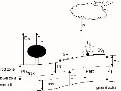
Figure 6.1.  Schematic representation of the different components of a soil water balance

Actual soil moisture content can be established according to (Driessen, 1986):

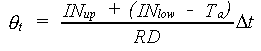(6.1a)

 

where		(6.1b)
and		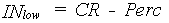(6.1c)

where	qt	:	Actual moisture content of the root zone at time step t	[cm3 cm-3]
	INup	:	Rate of net influx through the upper root zone boundary	[cm d-1]
	INlow	:	Rate of net influx through the lower root zone boundary	[cm d-1]
	Ta	:	Actual transpiration rate of crop	[cm d-1]
	RD	:	Actual rooting depth	[cm]
	P	:	Precipitation intensity	[cm d-1]
	Ie	:	Effective daily irrigation	[cm d-1]
	Es	:	Soil evaporation rate	[cm d-1]
	SSt	:	Surface storage	[cm]
	SR	:	Rate of surface runoff	[cm d-1]
	CR	:	Rate of capillary rise	[cm d-1]
	Perc	:	Percolation rate	[cm d-1]
	Dt	:	Time step	[d]
	Zt	:	Depth of groundwater table (see Figure 6.1.)	[cm]

The processes directly affecting the root zone soil moisture content can be defined as:

• infiltration: i.e. transport from the soil surface into the root zone;
• evaporation: i.e. the loss of soil moisture to the atmosphere;
• plant transpiration: i.e. loss of water from the interior root zone;
• percolation: i.e. downward transport of water from the root zone to the layer below the root zone;
• capillary rise: i.e. upward transport into the rooted zone.

The water balance equation has to be solved for each time interval in the crop growth cycle. For calculation of the potential production situation the soil moisture content is assumed to be at field capacity and the water balance is not simulated. For the water limited production situation two different soil water balances are distinguished. One without groundwater influence (i.e. for a freely draining soil) and one soil water balance with groundwater influence. In the JRC version due to lack pf data of WOFOST/CGMS, the system with groundwater is not activated, however, it can be easily applied whenever data are made available.

So, actually three water balance subroutines can be distinguished:

• Potential production [Section 6.2.]
• Water limited production, without groundwater influence [Section 6.3. ]
• Water limited production, with groundwater influence [Section 6.4.]

The actual canopy transpiration rate, used in the potential and water limited simulations, is calculated in a similar way for all options (See Section 6.1.). The capillary rise in the system with groundwater influence is a complicated subject. It will be discussed separately in Section 6.5..

In the water limited situation the water content of the root zone is the most important state variable, in- and outflow of water is calculated for each time step. It is important to realize that the model is not intended for detailed physical treatment of water movement in the soil, but only for estimating moisture availability to the crop. The distribution of water within the root zone is assumed to be instantaneous (within the time step of the model, being one day). The available water contained in the rooted zone is directly at the disposal of the crop. Water just below the root zone is available after further root growth. Water below the potential rooting depth cannot be used by the crop.

The infiltration process is not treated in a physical sense, because it would require a much smaller time step (Rietveld, 1978; Stroosnijder et al., 1972; van Keulen & van Beek, 1971). Instead a predefined fraction of the rain is not infiltrating on the day of rainfall (van Diepen et al., 1988).

Soil water content at saturation is equal to soil porosity. Field capacity is the volumetric water content of the soil after wetting and initial redistribution (Veihmeyer & Hendrickson, 1931). It is often treated as a soil characteristic (van Keulen, 1975; Driessen, 1986; Jansen & Gosseye, 1986), although it also depends on boundary conditions. Field capacity is usually defined as the volumetric water content at a soil moisture suction of 100 mbar or pF 2.0 at least in the Netherlands. It is the moisture suction in equilibrium with a groundwater table at 100 cm. Elsewhere in the world, for loamy soils field capacity corresponds with a value of 200 mbar moisture suction. For sandy soils 60 mbar is a realistic value under field conditions. Above a certain value of moisture suction, plants do not recover and wilt permanently. The volumetric soil water content at this point is called wilting point. The soil moisture at wilting point has usually a value of about 16000 mbar or pF 4.2. The soil moisture content of an air dry soil is assumed to be at pF 7.0 (van Keulen, 1975).
 
 

6.1. Evapo(transpi)ration

The following processes are calculated for a given crop cover (module CEvTra):

• The maximum evaporation rate from a shaded soil surface
• The maximum evaporation rate from a shaded water surface
• The maximum crop transpiration rate;
• The actual crop transpiration rate.

Transpiration, or the rate of water loss from plants depends on the energy available for vaporization, on the difference in vapor pressure between the plant and the surrounding air and on the resistance to water vapor diffusion from the stomatal cavity to the atmosphere (van Keulen & Seligman, 1987). Potential transpiration is the water loss from a field crop which covers the soil completely and has an optimum supply of water from the soil. The method, introduced by Penman (1956, 1948) and adapted according to Choisnel et al. (1992), is now used for daily totals of canopy transpiration and for daily totals of soil evaporation (Jarvis, 1981; Feddes et al., 1978; van Keulen, 1975).
 

Evaporation and transpiration

Potential crop evapotranspiration, ET0, is the sum of potential transpiration T_m and soil evaporation E0_s.

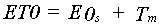(6.2)

Where	ET0	:	Potential evapotranspiration rate (see Section 4.1.4.)	[cm d-1]
	E0s	:	Potential evaporation of a bare soil (see Section 4.1.4.)	[cm d-1]
	Tm	:	Maximum crop transpiration rate (see eq. 6.4)	[cm d-1]

For some crops the potential evapotranspiration can be higher than the Penman evapotranspiration. Therefore, in the model a correction factor, a so called crop coefficient is introduced to account for this effect. The Penman evapotranspiration should be multiplied by this crop coefficient (Feddes, 1978; Doorenbos & Pruitt, 1977). The evaporation is reduced due to the presence of vegetation, which intercepts the solar energy and reduces the windspeed. The evaporation of the soil as a function of the leaf area index (Goudriaan, 1977; Ritchie, 1972; 1971) can be estimated as:

(6.3)

Where	E0s	:	Potential bare soil evaporation	[cm d-1]
	kgb	:	Extinction coefficient for global radiation	[-]
	LAI	:	Leaf area index	[ha ha-1]

The potential transpiration rate can be calculated by combining equations 6.2 and 6.3.

(6.4)

Where	Tm	:	Maximum crop transpiration rate	[cm d-1]
	ET0	:	Potential evapotranspiration rate	[cm d-1]
	kgb	:	Extinction coefficient for global radiation	[-]
	LAI	:	Leaf area index (see Section 5.5.5.)	[ha ha-1]

The extinction coefficient for global radiation can be estimated as a factor times the extinction coefficient of diffuse radiation:

(6.5)

Where	kgb	:	Extinction coefficient for global radiation	[-]
	kdf	:	Extinction coefficient for diffuse light	[-]

The maximum evaporation rate from a shaded water surface can be calculated in the same way as equation 6.4:

(6.6)

Where	Ew,max	:	Maximum evaporation rate from a shaded water surface	[cm d-1]
	E0w	:	Potential evaporation rate from a water surface (see Section 4.1.4.)	[cm d-1]
	kgb	:	Extinction coefficient for global radiation	[-]
	LAI	:	Leaf area index	[ha ha-1]

The maximum evaporation rate from a shaded bare soil surface can also be calculated in the same way as in equation 6.4 and 6.6:

(6.7)

Where	Es,max	:	Maximum evaporation rate from a shaded soil surface	[cm d-1]
	E0s	:	Potential evaporation rate from a bare soil surface	[cm d-1]
	kgb	:	Extinction coefficient for total global radiation	[-]
	LAI	:	Leaf area index	[ha ha-1]

 

Reduction of the transpiration due to water stress

For the potential situation the actual transpiration rate is always equal to the maximum transpiration rate: sufficient water is available. The actual transpiration rate is derived from the maximum transpiration rate, taking shortage or excess of water in the root zone into account. Water uptake by the roots depends on the difference in water potential in the plant and the soil and also on the resistance to moisture transport from the soil to the atmosphere (van Keulen & Seligman, 1987). In contrast to Feddes et al. (1978) not soil water potential, but soil water content is chosen as independent variable (Gollan et al., 1986; Schulze 1986).

Up to a point,a plant adapts its water potential to maintain potential transpiration. At what soil moisture content transition from potential transpiration to a transpiration deficit takes place, is difficult to quantify. The actual transpiration for the water limited situation is obtained by multiplying the potential transpiration with a reduction factor which is defined as (van Diepen et al., 1988):

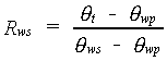(6.8)

Where	Rws	:	Reduction factor for transpiration in case of water shortage	[-]
	qt	:	Actual soil moisture content (see eq. 6.1 and 6.34)	[cm3 cm-3]
	qwp	:	Soil moisture content at wilting point	[cm3 cm-3]
	qws	:	Critical soil moisture	[cm3 cm-3]

 

The critical soil moisture content is defined as the quantity of stored soil moisture below which water uptake is impaired and the plant closes its stomata. It is not a fixed value. Restriction of water uptake due to water stress starts at a higher water content when the potential transpiration rate is higher (Denmead & Shaw, 1962). The critical moisture content can be calculated as (van Diepen et al., 1988):

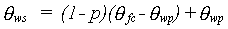(6.9)

Where	qws	:	Critical soil moisture content	[cm3 cm-3]
	p	:	Soil water depletion fraction as a function of pot. evapotranspiration	[cm3 cm-3]
	qfc	:	Soil moisture content at field capacity	[cm3 cm-3]
	qwp	:	Soil moisture content at wilting point	[cm3 cm-3]

 

Soil moisture content at field capacity,  q_fc, and the soil moisture content at wilting point, q_wp, are soil specific and should be given by the user. The soil water depletion fraction, p, is a function of the potential evapotranspiration rate (for a closed canopy) and crop group number. Instead of the term soil water depletion fraction, in literature also the expression easily available water is used which is defined as the water amount between q_fc and q_wp that can be extracted from the root zone without reducing the transpiration. Indicative p-values for the most important crops at different values of ET0 are presented in Table 6.1. Crop group number ranges from 1 (drought-sensitive) to 5 (drought-resistent). An example of a classification of the different crop groups is presented in Table 6.2.

Table 6.1. Soil water depletion fraction (p) as a function of potential evapotranspiration of a closed crop canopy for different crop groups (Doorenbos et al., 1978).

	ET0 in cm d-1
crop group	0.2	0.3	0.4	0.5	0.6	0.7	0.8	0.9	1.0
1	0.45	0.38	0.30	0.25	0.23	0.20	0.18	0.16	0.15
2	0.60	0.50	0.43	0.35	0.30	0.28	0.25	0.23	0.20
3	0.75	0.65	0.55	0.45	0.40	0.38	0.33	0.30	0.25
4	0.85	0.75	0.65	0.55	0.50	0.48	0.43	0.38	0.35
5	0.92	0.85	0.75	0.65	0.60	0.55	0.50	0.48	0.45

 

Table 6.2. Example of crops in the different crop groups (Doorenbos et al., 1978).

1	leaf vegetables, strawberry	1-2	cabbage, onion
2	clover, carrot, early tobacco	2-3	banana, pepper
3	grape, pea, potato	3-4	bean, sunflower, tomato, water melon, grass
4	citrus, groundnut, pineapple	4-5	alfalfa cotton, tobacco, cassava, sweet potato, grains
5	olive, safflower, sorghum, soybean, sugarcane

 

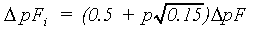
The soil water depletion fraction for very high values of potential evapotranspiration of a closed canopy can be as low as 0.10. For very low values of potential evapotranspiration of a closed canopy this fraction can reach 0.96. Note that the reduction factor R_ws (eq. 6.8) may obtain values higher than unity and lower than zero for certain values of p and q_t. Since this does not make any sense, in WOFOST/CGMS the highest possible value for R_ws is set to unity and the lowest possible value to zero. An empirical formula can be used to calculate the fraction of easily available soil water, yielding identical values as the ones given in the Table 6.1. (van Diepen et al., 1988).

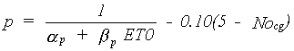(6.10)

where	p	:	Fraction of easily available soil water	[cm3 cm-3]
	ap	:	Regression constant (=0.76 van Diepen et al., 1988)	[-]
	bp	:	Regression constant (=1.5 van Diepen et al., 1988)	[d cm-1]
	ET0	:	Potential evapotranspiration rate	[cm d-1]
	Nocg	:	Crop Group number (=1 to 5, Doorenbos et al., 1978)	[-]

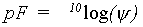
Note that crop group number, No_cg should be provided by the user. For crop group 1 and 2 this estimate is not very accurate and an additional correction is applied to reproduce the table values correctly (van Diepen et al., 1988):

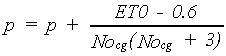(6.11)

where	p	:	Fraction of easily available soil water	[cm3 cm-3]
	ET0	:	Potential evapotranspiration rate	[cm d-1]
	Nocg	:	Crop Group number (=1 to 5, Doorenbos et al., 1978)	[-]

 

Reduction of the transpiration due to oxygen stress

The plant transpiration rate can also be reduced when the rootzone is completely saturated. Root systems which have been developed in aerobic soils do not have airducts and degenerate within several days when anaerobic conditions (waterlogging) are imposed (Penning de Vries et al., 1989). Flooding quickly depletes the O₂ in the soil and root cells disintegrate when their metabolic activities are hampered by oxygen depletion. For detailed information on the physiological effects of excess water on a crop see Jackson and Drew (1984).Transpiration reduction occurs when the actual soil moisture content exceeds the critical soil moisture content for aeration. The critical soil moisture content for aeration can be calculated as:

(6.12)

Where	qair	:	Critical soil moisture content for aeration	[cm3 cm-3]
	qmax	:	Soil porosity	[cm3 cm-3]
	qc	:	Critical air content	[cm3 cm-3]

The soil porosity, q_max, and the critical soil air content, q_c, are soil specific and should be provided by the user. In WOFOST/CGMS maximum reduction is reached after four successive days of anaerobic conditions. In reality however, this period depends on the development stage and species. The transpiration rate reduction factor due to oxygen shortage can be calculated as (van Diepen, personal communication):

	(6.13a)
	(6.13b)

Where	Ros,max	:	Maximum reduction factor due to oxygen shortage	[-]
	Ros	:	Reduction factor due to oxygen shortage	[-]
	qair	:	Critical soil moisture content for aeration	[cm3 cm-3]
	qmax	:	Soil porosity	[cm3 cm-3]
	qt	:	Actual soil moisture content (see eq. 6.34)	[cm3 cm-3]
	Nod	:	Number of successive days with oxygen stress	[-]

 

For crops which roots develop airducts (e.g rice) and for crops grown on perfectly drained land, the reduction factor for oxygen shortage equals unity. If this ratio is less then unity, the actual transpiration rate is reduced proportionally. Usually, in freely draining soils oxygen stress does not play any role. However, it may occur when (i) the critical soil moisture content for aeration is greater than the soil moisture content at field capacity, when (ii) the subsoil is very slowly permeable and when (iii) a high groundwater table occurs (in this in case oxygen shortage may occur regularly). However, the process of transpiration reduction due oxygen shortage is poorly parametrized and values for the reduction factor are rather speculative.
 

Actual transpiration

As a result of water excess and/or water shortage the actual transpiration rate can be calculated as:

(6.14)

Where	Ta	:	Actual transpiration rate	[cm d-1]
	Tm	:	Maximum transpiration rate (see eq. 6.4)	[cm d-1]
	Ros	:	Reduction factor due to oxygen reduction	[-]
	Rws	:	Reduction factor due to water shortage (see eq. 6.8)	[-]

 
 

6.2. Soil water balance calculations, potential production

To quantify the crop water requirements for continuous growth without drought stress (i.e. assuming that the soil is permanently at field capacity) the variables of the soil water balance in the potential production situation are calculated.

(6.15)

Where	qt	:	Actual soil moisture content	[cm3 cm-3]
	qfc	:	Soil moisture content at field capacity	[cm3 cm-3]

Rainfall, irrigation, capillary rise and drainage are not taken into account. This does not mean that these processes will not occur. The result of these processes will be a soil moisture content at field capacity level. The only two processes to consider are surface evaporation and crop transpiration (see the previous sections).

The evaporation rate is calculated for two situations:

• Airducts are present in the roots and the crop tolerates waterlogging (e.g. rice). The evaporation rate is then calculated as the evaporation rate from a shaded water surface:

(6.16)

Where	Ew	:	Evaporation rate from a shaded water surface	[cm d-1]
	Ew,max	:	Maximum evaporation rate from shaded water surface (see eq. 6.6)	[cm d-1]

• Airducts are absent in the roots and the crop does not tolerate water logging (most crops). The evaporation rate is calculated as the evaporation rate from a soil surface (van Diepen, personal communication):

(6.17)

Where	Es	:	Evaporation rate from a shaded soil surface	[cm d-1]
	Es,max	:	Maximum evaporation rate from a shaded soil surface (see eq. 6.7)	[cm d-1]
	qfc	:	Soil moisture content at field capacity	[cm3 cm-3]
	qwp	:	Soil moisture content at wilting point	[cm3 cm-3]
	qmax	:	Soil porosity	[cm3 cm-3]

 
 

6.3. System without groundwater influence

In subroutine Calculate, the variables of the soil water balance in the actual water-limited production situation are calculated for freely draining soil. No influence from groundwater is assumed and crop water requirements for continuous growth with either drought stress or water excess and a possible reduction of the crop transpiration rate, leading to a reduced growth are quantified.
 
 

6.3.1. The soil water submodel

For the rooted zone the water balance equation is solved every daily time step. The water balance is driven by rainfall, possibly buffered as surface storage, and evapotranspiration. The processes considered are infiltration, soil water retention, percolation and the loss of water beyond the maximum root zone. At the upper boundary, processes comprise infiltration of water from precipitation or irrigation, evaporation from the soil surface and crop transpiration. If the rainfall intensity exceeds the infiltration and surface storage capacity of the soil, water runs off. Water can be stored in the soil till the field capacity is reached. Additional water percolates beyond the lower boundary of the rooting zone. Flow rates are limited by the maximum percolation rate of the root zone and the maximum percolation rate to the subsoil. The textural profile of the soil is conceived homogeneous. Initially the soil profile consists of three layers (zones):

• the rooted zone between soil surface and actual rooting depth
• the lower zone between actual rooting depth and maximum rooting depth
• the subsoil below maximum rooting depth

Root zone extension from initial rooting depth to maximum rooting depth is described in Section 5.6. Its effect on the soil moisture content is accounted for in this soil water balance calculation. From the moment that the maximum rooting depth is reached the soil profile is described as a two layer system (Driessen, 1986). The lower zone no longer exists. As mentioned earlier, no groundwater influence is assumed and capillary rise is not accounted for. Only downward flow, evaporation from the soil surface and transpiration are estimated.
 
 

6.3.2. Elements of the water balance

Initial soil water content and initial soil water amount

The initial value of the actual soil moisture content in the root zone can be calculated as:

(6.18)

Where	qt	:	Actual soil moisture content in rooted zone	[cm3 cm-3]
	qwp	:	Soil moisture content at wilting point	[cm3 cm-3]
	Wav	:	Initial available soil moisture amount in excess of qwp	[cm]
	RD	:	Actual rooting depth (see Section 5.6.)	[cm]

The initial actual soil moisture content, q_t, cannot be lower than the soil moisture content at wilting point. In case the crop cannot develop airducts, the initial soil moisture content cannot be higher than the soil moisture content at field capacity. If the crop can develop airducts the initial soil moisture content cannot exceed the soil porosity. W_av, the initial available soil moisture amount in excess of q_wp should be provided by the user. Multiplying the actual soil moisture content with the rooting depth yields the initial water amount in the rooted zone. The initial amount of soil moisture in the zone between the actual rooting depth and the maximum rooting depth (i.e. lower zone), can be calculated as:

(6.19)

Where	Wlz	:	Soil moisture amount in the lower zone	[cm]
	Wav	:	Initial available soil moisture amount in excess of qwp	[cm]
	RDmax	:	Maximum rooting depth	[cm]
	RD	:	Actual rooting depth	[cm]
	qt	:	Actual soil moisture content in rooted zone	[cm3 cm-3]
	qwp	:	Soil moisture content at wilting point	[cm3 cm-3]

The soil moisture content of the lower zone is also limited by the field capacity in case the crop cannot develop airducts, else the soil moisture content is limited by the soil porosity. In WOFOST/CGMS, the variable D_slr, days since last rain, is initially set to one. If the actual soil moisture content is halfway between the field capacity and wilting point a value of five days is assumed.
 

Evaporation

Evaporation depends on the available soil water and the infiltration capacity of the soil. If the water layer on the surface, the so called surface storage, exceeds 1 cm, the actual evaporation rate from the soil is set to zero and the actual evaporation rate from the surface water is equal to the maximum evaporation from a shaded water surface. If the surface storage is less than 1 cm and the infiltration rate of the previous day exceeds 1 cm d^-1, the actual evaporation rate from the surface water is set to zero and the actual evaporation rate from the soil is equal to the maximum evaporation from a shaded soil surface. All water on the surface can infiltrate within one day. The value of the variable days since last rain, D_slr, is reset to unity. If the infiltration rate is less than 1 cm d^-1, the amount of infiltrated water is considered too small to justify a reset of the parameter D_slr and the evaporation rate decreases as the top soil starts drying. The reduction of the evaporation is thought to be proportional to the square root of time (Stroosnijder, 1987, 1982). The evaporation can be calculated as:

(6.20)

where	Es	:	Evaporation rate from a shaded soil surface	[cm d-1]
	Es,max	:	Maximum evaporation rate from a shaded soil surface (see eq. 6.7)	[cm d-1]
	Dslr	:	Days since last rain	[d]

When a small water amount has infiltrated, or rather wetted the soil surface, this amount can be evaporated the same day, irrespective of D_slr. Therefore, the actual evaporation from the soil surface, as calculated according to equation 6.20, should be corrected for this water amount infiltrating the soil. This amount should be added to the actual evaporation rate. However, it should be noted that the actual evaporation can never exceed the maximum evaporation rate.
 

Precipitation

Not all precipitation will reach the surface. A fraction will be intercepted by leaves, stems, etc. From the amount of precipitation which reaches the soil surface, a part runs off. Runoff from a field can be 0-20 percent, and even higher on unfavorable surfaces (Stroosnijder & Koné, 1982). WOFOST/CGMS assumes that a fixed fraction of the precipitation will not infiltrate during that particular day. This fraction can be reduced in situations with relatively small amounts of rainfall. The reduction factor is defined as function of the rainfall amount (van Diepen et al., 1988). See figure 6.2 and equation 6.26. Note that the non infiltrating fraction refers to rainfall only. Irrigation water is assumed to infiltrate freely (the irrigation option is not implemented in WOFOST/CGMS).

 

Figure 6.2. Reduction factor of the non infiltrating fraction as a function of rainfall.
 

Percolation

If the root zone soil moisture content is above field capacity, water percolates to the lower part of the potentially rootable zone and the subsoil. A clear distinction is made between percolation from the actual rootzone to the so-called lower zone, and percolation from the lower zone to the subsoil. The former is called Perc and the latter is called Loss. The percolation rate from the rooted zone can be calculated as:

(6.21)

where	Perc	:	Percolation rate from the root zone to the lower zone	[cm d-1]
	Wrz	:	Soil moisture amount in the root zone (see eq. 6.33a)	[cm]
	Wrz,fc	:	Equilibrium soil moisture amount in the root zone (see eq. 6.22)	[cm]
	Dt	:	Time step	[d]
	Ta	:	Actual transpiration rate (see eq. 6.14)	[cm d-1]
	Es	:	Evaporation rate from a shaded soil surface (see eq. 6.7 and 6.20)	[cm d-1]

The equilibrium soil moisture amount in the root zone can be calculated as the soil moisture content at field capacity times the depth of the rooting zone:

(6.22)

where	Wrz,fc	:	Equilibrium soil moisture amount in the root zone	[cm]
	qfc	:	Soil moisture content at field capacity	[cm3 cm-3]
	RD	:	Actual rooting depth	[cm]

The percolation rate and infiltration rate are limited by the conductivity of the wet soil, which is soil specific and should be given by the user. Note that the percolation from the root zone to the lower zone can be limited by the uptake capacity of the lower zone. Therefore, the value calculated with equation 6.21 is preliminary and the uptake capacity should first be checked. The percolation from the lower zone to the subsoil, the so-called Loss, should take the water amount in the lower zone into account. If the water amount in the lower zone is less than the equilibrium soil moisture amount, a part of the percolating water will be retained and the percolation rate will be reduced. Water loss from the lower end of the maximum root zone can be calculated as:

(6.23)

where	Loss	:	Percolation rate from the lower zone to the subsoil	[cm d-1]
	Perc	:	Percolation rate from root zone to lower zone (see eq. 6.21)	[cm d-1]
	Wlz	:	Soil moisture amount in the lower zone (see eq. 6.33b)	[cm]
	Wlz,fc	:	Equilibrium soil moisture amount in the lower zone (see eq. 6.24)	[cm]
	Dt	:	Time step

Water loss from the potentially rootable zone, is also limited by the maximum percolation rate of the subsoil, which is soil specific and should be provided by the user. The equilibrium soil moisture amount in the lower zone can be calculated as the soil moisture content at field capacity times the root zone depth:

(6.24)

where	Wrz,fc	:	Equilibrium soil moisture amount in the lower zone	[cm]
	qfc	:	Soil moisture content at field capacity	[cm3 cm-3]
	RDmax	:	Maximum rooting depth	[cm]
	RD	:	Actual rooting depth	[cm]

For rice an additional limit of five percent of the saturated soil conductivity is set to account for puddling (a rather arbitrary value, which may be easily changed in the program). The saturated soil conductivity and is calculated using equating 6.67 with pF= -1.0 (i.e. a hydraulic head of 0.1 cm). The percolation rate from the lower zone to the sub soil is not to exceed this value (van Diepen et al., 1988). As mentioned before, the value calculated with equation 6.21, should be regarded as preliminary; the storage capacity of the receiving layer may become limiting. The storage capacity of the lower zone, also called the uptake capacity, is the amount of air plus the loss (van Diepen et al., 1988). It can de defined as:

(6.25)

where	UP	:	Uptake capacity of lower zone	[cm d-1]
	RDmax	:	Maximum rooting depth	[cm]
	RD	:	Actual rooting depth	[cm]
	Wlz	:	Soil moisture amount in lower zone	[cm]
	qmax	:	Soil porosity (maximum soil moisture)	[cm3 cm-3]
	Dt	:	Time step	[d]
	Loss	:	Percolation rate from the lower zone to the subsoil	[cm d-1]

Percolation to the lower part of the potentially rootable zone can not exceed the uptake capacity of the lower zone. Therefore the percolation rate is set equal to the minimum of the calculated percolation rate (eq. 6.21) and the uptake.
 

Preliminary infiltration

The infiltration rate depends on the available water and the infiltration capacity of the soil. If the actual surface storage is less then or equal to 0.1 cm, the preliminary infiltration capacity is simply described as:

(6.26)

where	INp	:	Preliminary infiltration rate	[cm d-1]
	FI	:	Maximum fraction of rain not infiltrating during time step t	[-]
	CI	:	Reduction factor applied to FI as a function of the precipitation intensity	[-]
	P	:	Precipitation intensity	[cm d-1]
	Ie	:	Effective irrigation	[cm d-1]
	SSt	:	Surface storage at time step t (see eq. 6.29)	[cm]
	Dt	:	Time step	[d]

The maximum fraction of rain not infiltrating during time step t, F_I can be either set to a fixed value or assumed to be variable by multiplying F_I with a precipitation dependent reduction factor C_I which is maximum for high rainfall and will be reduced for low rainfall. The user should provide F_I. The C_I table is included in the model and is assumed to be fixed. The calculated infiltration rate is preliminary, as the storage capacity of the soil is not yet taken into account. If the actual surface storage is more than 0.1 cm, the available water which can potentially infiltrate, is equal to the water amount on the surface (i.e. supplied via rainfall/irrigation and depleted via evaporation):

(6.27)

where	INp	:	Preliminary infiltration rate	[cm d-1]
	P	:	Precipitation intensity	[cm d-1]
	Ie	:	Effective irrigation	[cm d-1]
	Ew	:	Evaporation rate from a shaded water surface	[cm d-1]
	SSt	:	Surface storage at time step t (see eq. 6.29)	[cm]
	Dt	:	Time step	[d]

However, the infiltration rate is hampered by the soil conductivity and cannot exceed it. Soil conductivity is soil specific and should be given by the user.
 

Adjusted infiltration

Total water loss from the root zone can now be calculated as the sum of transpiration, evaporation and percolation. The sum of total water loss and available pore space in the root zone define the maximum infiltration rate. The preliminary infiltration rate cannot exceed this value. The maximum possible infiltration rate is given by:

(6.28)

where	INmax	:	Maximum infiltration rate	[cm d-1]
	qmax	:	Soil porosity (maximum soil moisture)	[cm3 cm-3]
	qt	:	Actual soil moisture content	[cm3 cm-3]
	RD	:	Actual rooting depth	[cm]
	Dt	:	Time step	[d]
	Ta	:	Actual transpiration rate	[cm d-1]
	Es	:	Evaporation rate from a shaded soil surface	[cm d-1]
	Perc	:	Percolation rate from root zone to lower zone	[cm d-1]

 

Surface runoff

Surface runoff is also taken into account by defining a maximum value for surface storage. If the surface storage exceeds this value the exceeding water amount will run off. Surface storage at time step t can be calculated as:

(6.29)

where	SSt	:	Surface storage at time step t	[cm d-1]
	P	:	Precipitation intensity	[cm d-1]
	Ie	:	Effective irrigation rate	[cm d-1]
	Ew	:	Evaporation rate from a shaded water surface	[cm d-1]
	IN	:	Infiltration rate (adjusted)	[cm d-1]

Surface runoff can be calculated as:

(6.30)

where	SRt	:	Surface runoff at time step t	[cm]
	SSt	:	Surface storage at time step t	[cm]
	SSmax	:	Maximum surface storage	[cm]

SS_max is an environmental specific variable and should be provided by the user.
 

Rates of change and root extension

The rates of change in the water amount in the root and lower zone are calculated straightforward from the flows found above:

	(6.31a)
	(6.31b)

where	DWrz	:	Change of the soil moisture amount in the root zone	[cm]
	DWlz	:	Change of the soil moisture amount in the lower zone	[cm]
	Ta	:	Actual transpiration rate	[cm d-1]
	Es	:	Evaporation rate from a shaded soil surface	[cm d-1]
	IN	:	Infiltration rate	[cm d-1]
	Perc	:	Percolation rate from root zone to lower zone	[cm d-1]
	Loss	:	Percolation rate from lower zone to sub soil	[cm d-1]
	Dt	:	Time step	[d]

Due to extension of the roots into the lower zone, extra soil moisture becomes available, which can be calculated as:

(6.32)

where	RDt	:	Rooting depth at time step t	[cm]
	RDt-1	:	Rooting depth at time step t-1	[cm]
	RDmax	:	Maximum rooting depth	[cm]
	Wlz	:	Soil moisture amount in the lower zone (see eq. 6.33b)	[cm]
	DWrz	:	Change of the soil moisture amount in the root zone	[cm]
	DWlz	:	Change of the soil moisture amount in the lower zone	[cm]

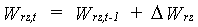
With equation 6.31 the actual water amount in the root zone and in the lower zone can be calculated according to:

	(6.33a)
	(6.33b)

where	Wrz,t	:	Soil moisture amount in the root zone at time step t	[cm]
	Wlz,t	:	Soil moisture amount in the lower zone at time step t	[cm]
	Wrz,t-1	:	Soil moisture amount in the root zone at time step t-1	[cm]
	Wlz,t-1	:	Soil moisture amount in the lower zone at time step t-1	[cm]
	DWrz	:	Rate of change of the soil moisture amount in the root zone	[cm]
	DWlz	:	Rate of change of the soil moisture amount in the lower zone	[cm]

 

Actual soil moisture content

The actual soil moisture content can now be calculated according to (see also eq. 6.1):

(6.34)

where	qt	:	Actual soil moisture content at time step t	[cm3 cm-3]
	Wrz,t	:	Soil moisture amount in the root zone at time step t	[cm]
	RD	:	Actual rooting depth	[cm]

 
 

6.4. Subsystem with groundwater influence

Crop water requirements are quantified for continuous growth with either drought stress or water excess and a possible reduction of the crop transpiration rate, leading to a reduced growth, is quantified. Note that the routines discussed in the following sections are not included in CGMS!
 
 

6.4.1. Submodel with groundwater influence

The textural soil profile is assumed to be homogeneous and three zones are distinguished:

• the rooted zone between soil surface and actual rooting depth
• the zone between rooting depth and groundwater
• the soil below groundwater level to a reference depth of 1000 centimeters. This reference depth is used to calculate a system water balance. It is a formal system boundary

Root zone extension is described in Section 5.6. and is considered in the soil water balance calculation. When the maximum rooting depth is reached the soil profile is described as a two layer system: the lower zone no longer exists. Two situations are distinguished: (i) with artificial drainage and (ii) without artificial drainage. The soil water balance estimates the daily value of the mean soil moisture content for a cropped field (water limited situation only). The soil moisture content influences water uptake and crop transpiration and thus the assimilation (see eq. 5.33).

The water balance is driven by rainfall, possibly buffered as surface storage and evapotranspiration. The processes considered are infiltration, soil water retention, the steady state flow between the root zone and the groundwater table (capillary rise() or percolation(), and drainage rate. An irrigation term is included but not used. The resulting depth, moisture and air contents in the root zone are calculated. Calculation of the evaporation rate, the preliminary infiltration rate, precipitation, surface storage and runoff is similar to the system without groundwater influence (see prevous sections).

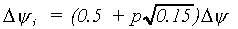
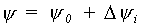
Groundwater influence is taken into account by calculation of capillary rise assuming a stationary situation and homogeneous soil. The time step of one day implies that some of the calculated flow rates may result in moisture contents exceeding the total pore space. This clearly sets a limit to the values of these rates of change. As a consequence, the model has more or less the character of a bookkeeping system. The rate of capillary rise or percolation determine the change in groundwater level. The new groundwater level is thus estimated from the calculated capillary rise or percolation. The soil moisture profile in the soil between groundwater and rooted zone, is assumed to be again in equilibrium. (in fact a contradiction with capillary rise or percolation). Difficulty arises when the groundwater rises into the rooted zone. The following procedure is then applied:

• To simplify the calculations, it is assumed that in the current time step the groundwater can rise until the lower boundary of the rooted zone at its highest level.
• Soil air content of the rooted zone is calculated in next step. If the water amount in the rooted zone increases, a lower, saturated layer and a higher layer with the original air content and soil moisture content are assumed and the groundwater table is situated at the boundary between these zones. The root zone may be completely filled (groundwater level equals zero).
• Water loss from the rooted zone implies a rise of the groundwater level and the increase of soil moisture in the zone between groundwater and root zone is considered as capillary rise. At the other hand the groundwater level may drop below the rooted zone due to water loss.

No capillary flow occurs if the groundwater table is within the root zone. The simulation stops when the following circumstances arise:

• waterlogging occurs (i.e. groundwater depth less then 10 cm) and the plants cannot form airducts.
• plants can form airducts but waterlogging prevails for more then ten consecutive days.

 

6.4.2. Root extension and the actual soil moisture content

The elements of the water balance have to be established before the actual soil moisture content can be calculated. In the following paragraph percolation, capillary rise, adjusted infiltration and actual soil moisture amount are discussed. The new level of the groundwater table, which is needed to calculate the capillary rise, is also established. The effect of root extension will be explained at the end of this paragraph.
 

Initialization

Some remarks have to be made on the initialization: the soil moisture content values at field capacity, wilting point and the soil porosity are derived from the water retention curve, q _log(y) (see eq. 6.38). An AFGEN table with the ¹⁰log of the matric head (pF) as independent variable is used to describe this curve. The water retention curve is soil specific and should be provided by the user. Soil moisture content at field capacity, q_fc, soil moisture content at wilting point, q _wp and soil porosity, q_max are established using the AFGEN table mentioned above with a matric head of 200 cm, 16000 cm and 0.1 cm respectively. In WOFOST a pF table is constructed as the inverse of q _log(y).

First, a table with values of the cumulative soil air volume above the groundwater level at equilibrium is calculated. Under equilibrium conditions, the matric head values are numerically equal to the height at which they occur. With soil air volume, the cumulative air amount as a function of height above groundwater under equilibrium conditions is meant. Values of the cumulative air amount for the following values of height (matric head, also called soil suction): 0,2,4,8,16,32,64,128,..,16384 cm are calculated and put into an AFGEN table. To calculate the cumulative air amount, the soil air content has to be integrated over the intervals mentioned above. The three point Gaussian integration method is used in the model. Length of the integration interval is given by:

(6.35)

where	Dy	:	Height of interval matric head	[cm]
	y0	:	Lower boundary interval matric head	[cm]
	y1	:	Upper boundary interval matric head	[cm]

Within each interval, three points are selected and used by the Gaussian integration, to integrate over the interval are given by:

(6.36)

where	yi	:	Matric head	[cm]
	p	:	Three points for Gaussian integration	[-]

Average air content for the selected matric head can be calculated as:

(6.37)

where	qair,yi	:	Air content at selected matric head	[cm3 cm-3]
	qmax	:	Soil porosity	[cm3 cm-3]
	qyi	:	Actual soil moisture content as a function of matric head	[cm3 cm-3]

The actual soil moisture content can be derived as a function of the selected matric head using the soil specific water retention curve:

(6.38)

where	qyi	:	Actual soil moisture content as a function of matric head	[cm3 cm-3]
	Dy	:	Height of interval matric head	[cm]
	y0	:	Lower boundary interval matric head	[cm]

With equations 6.35, 6.36, 6.37 and 6.38, the cumulative air amount as a function of height above groundwater under equilibrium conditions can now be calculated as:

(6.39)

where	Aair(h)	:	Air amount as a function of height (h) above groundwater table	[cm]
	Dy	:	Height of interval matric head	[cm]
	qair,p	:	Air content at selected matric head p=-1,0,1	[cm3 cm-3]

The AFGEN table, the matric head (or height above groundwater) as a function of the cumulative air amount, y(A_air), is also calculated. It is the inverse of the table calculated above.

With equation 6.39, the soil air amount above the water table at equilibrium, the initial state variables of the water balance can be computed. These are, the equilibrium moisture amount in the subsoil, in the root zone and the zone above the drains up to the surface. Before this can be done however, the soil air volume below the rooted zone, in the root zone and above the drains up to the surface has to be established. To estimate the air amount at a specific depth at equilibrium, the height of that specific level above soil water table is used. It is assumed that in the rootzone no gradient exists.

The equilibrium moisture amount in the subsoil, the root zone and above the drains up to the surface can than be calculated as:

	where:		(6.40a)
	where:		(6.40b)
	where:		(6.40c)

where	Wss,fc	:	Equilibrium soil moisture amount below rooted zone	[cm]
	Wrz,fc	:	Equilibrium soil moisture amount in rooted zone	[cm]
	Wdd,fc	:	Equilibrium soil moisture amount above the drains up to the surface	[cm]
	Aair(h)	:	Air amount as a function of height above groundwater table (see eq. 6.39)	[cm]
	qmax	:	Soil porosity	[cm3 cm-3]
	RD	:	Actual rooting depth	[cm]
	DD	:	Drain depth	[cm]
	Zt	:	Depth of groundwater table at time step t	[cm]

The initial moisture content in the rooted zone is assumed to be equal to the equilibrium moisture amount in the root zone if the groundwater level is within 100 cm from the root zone or even in the root zone. If the groundwater level is lower than 100 cm below the root zone the initial moisture content in the rooted zone is calculated as the soil moisture at field capacity. The variable days since last rain, D_slr, which is used to calculate the evaporation rate from a shaded soil (see eq. 6.20), is set to unity. In case the soil moisture is lower than pF 3.0, a value of five days is assumed.
 

Capillary rise and percolation

If the groundwater level is within the root zone, capillary rise and percolation are set to zero and no capillary rise or percolation has to be calculated. If the groundwater level is below the root zone, both capillary rise and percolation are calculated. The capillary flow from groundwater to the root zone is calculated from the pF of the root zone, the height difference between the lower boundary of the root zone and the groundwater depth and the table of the hydraulic conductivity. The pF can be derived via interpolation from the soil specific water retention curve. Because of its complex calculations, capillary flow is discussed separately in Section 6.5..

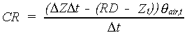
For sandy soils, a shallow groundwater depth and a shallow root zone, the capillary flow may be so large that the system becomes unstable. Therefore, the calculated flow rate is limited to the flow rate that would exist in a state of equilibrium with the groundwater level, which can be calculated as:

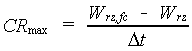(6.41)

where	CRmax	:	Maximum flow rate calculated at equilibrium	[cm d-1]
	Wrz,fc	:	Equilibrium water amount in the rooted zone (see eq. 6.40b)	[cm]
	Wrz	:	Actual water amount in the rooted zone (see eq. 6.55)	[cm]
	Dt	:	Time step	[d]

A positive flow rate is defined as capillary rise whereas a negative flow rate is considered as percolation. For rice crops the percolation is limited to 5% of the estimated soil specific hydraulic conductivity, to account for the effect of puddling. This is a rather arbitrary value.
 

Drainage

The drainage rate is calculated only if there artificial drainage exists and if the groundwater level is above the drainage depth. For other cases the drainage depth is set to zero. The drainage rate depends on the drainable water amount and the drainage system capacity. This capacity is calculated first accorrding to (van Diepen et al., 1988):

(6.42)

where	DRmax	:	Maximum drainage rate, equal to the drainage capacity	[cm d-1]
	K0	:	Hydraulic conductivity at saturation	[cm d-1]

The hydraulic conductivity at saturation, K0 is soil specific and is calculated using equating 6.67 with pF= -1.0 (i.e. a matric head of 0.1 cm). If the groundwater table is below the root zone the drainable water amount equals the water amount water between the drains and the root zone minus the equilibrium amount which corresponds with the groundwater level at drainage depth. It is assumed that the drainage rate is always positive or zero (in case RD > DD and W_rz < W_dd,fc).
The drain depth, should be given be the user. The drainage rate can be calculated as:

(6.43)

where	DR	:	Drainage rate	[cm d-1]
	Wrz	:	Water amount in the root zone (see eq. 6.55)	[cm]
	DD	:	Drain depth	[cm]
	RD	:	Actual rooting depth	[cm]
	qmax	:	Soil porosity	[cm3 cm-3]
	Wdd,fc	:	Water amount above drains (see eq. 6.40c)	[cm]
	Dt	:	Time step	[d]

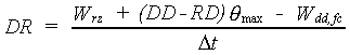
For groundwater located within the root zone the drainable water amount equals the water content of the root zone plus the water content of the (saturated) zone between the drains and the rootzone, minus the equilibrium water amount above the drains. The drainage rate can be calculated as:

(6.44)

where	DR	:	Drainage rate	[cm d-1]
	h2	:	Zt - RD	[cm]
	h1	:	DD - RD	[cm]
	Aair(h)	:	Air amount as a function of height above groundwater table (see eq. 6.39)	[cm]
	DD	:	Drain depth	[cm]
	RD	:	Actual rooting depth	[cm]
	Zt	:	Groundwater table depth at time step t	[cm]
	Dt	:	Time step	[d]

Note that the drainage rate cannot exceed the drainage capacity of the system (eq. 6.42)
 

Change of groundwater depth and adjustment of infiltration rate

In the following text, the change of the groundwater and the adjustment of the infiltration rate will be discussed. Two different situations can be distinguished.

• Groundwater table below the rooted zone
• Groundwater table within the rooted zone

In case the groundwater table is within the rooted zone, the water table may drop below the rooted zone. To maintain a stable moisture content in the model, water is recovered from the subsoil. This water amount is accounted for as capillary rise in the water balance of the rooted zone.

Groundwater table below rootzone

Now the change in groundwater depth and the infiltration rate can be adjusted. If the groundwater level is below the root zone the calculation is simple. From the drainage rate, the rate of capillary rise and/or percolation rate, the new air amount between root zone and groundwater can be found:

(6.45)

where	Anew	:	New air amount between root zone and groundwater level	[cm]
	Aair(h)	:	Air amount as a function of height above groundwater table (see eq. 6.39)	[cm]
	h	:	Zt - RD	[cm]
	RD	:	Actual rooting depth	[cm]
	Zt	:	Depth of groundwater table at time step t	[cm]
	DR	:	Drainage rate	[cm d-1]
	CR	:	Rate of capillary rise (see Section 6.5.)	[cm d-1]
	Perc	:	Percolation rate	[cm d-1]

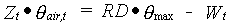
To simplify calculations, the groundwater is not allowed to enter the root zone in the current time step. This may happen when the new air amount between ground-water and root zone, A_new, becomes negative. The groundwater level is allowed to rise maximally till the lower boundary of the root zone (A_new=0). In the next time step the groundwater may rise further. Therefore, the percolation rate is constrained to prevent such an occasion.

(6.46)

where	Perc	:	Percolation rate	[cm d-1]
	Anew	:	New air amount between root zone and groundwater table	[cm]
	Dt	:	Time step	[d]

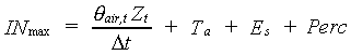
The definitive percolation value is now known and used to constrain the maximum possible infiltration rate (to prevent an over saturated root zone), which equals the available soil air volume:

(6.47)

where	INmax	:	Maximum infiltration rate	[cm d-1]
	qmax	:	Soil porosity	[cm3 cm-3]
	qt	:	Soil moisture content (see eq. 6.56)	[cm3 cm-3]
	RD	:	Actual rooting depth	[cm]
	Dt	:	Time step	[d]
	Ta	:	Actual transpiration	[cm d-1]
	Es	:	Evaporation rate of shaded soil surface	[cm d-1]
	Perc	:	Percolation rate	[cm d-1]
	CR	:	Rate of capillary rise	[cm d-1]

The root zone soil moisture content is limited to a value just below saturation to prevent zero air content in the root zone, which could lead to problems in the next time step if, at that day, the groundwater enters the rooted zone. The adjusted infiltration rate (see eq. 6.26 and 6.27) is established by limiting the preliminary infiltration to maximum possible infiltration rate.

The equilibrium profile is assumed and the new height of the root zone above the groundwater level (i.e. matric head at the root tip) can now be obtained from the relation between height above the groundwater table and the cumulative air amount y(A_air), by introducing the new air amount between the root zone and the groundwater level, A_new, into this relation. Adding the actual rooting depth, RD, yields the groundwater depth. The rate of change of the groundwater level is found by subtracting the old value of the groundwater depth from the new value.

(6.48)

where	DZ	:	Change in groundwater level per time step	[cm d-1]
	y()	:	Matric head as a function of the air amount	[cm]
	Anew	:	New air amount between root zone and groundwater level (see eq. 6.45)	[cm]
	RD	:	Actual rooting depth	[cm]
	Zt-1	:	Depth of groundwater table at time step t-1	[cm]

The initial groundwater depth should be provided by the user.
 

Groundwater table within the rooted zone

When groundwater enters the rooted zone, the air concentration in the root zone is calculated. Percolation is assumed to equal the maximum drainage rate. The root zone is divided into a part saturated with water and an unsaturated part. The initial air concentration is maintained in the unsaturated part. This implies that an increase of the water content leads to a shallower unsaturated part and hence to a rising groundwater level.

This rather artificial construction is necessary because of the inter-dependence of the water content and the groundwater depth. In this system the relation between water content and groundwater depth is (van Diepen et al., 1988):

(6.49)

where	Zt	:	Depth of groundwater table at time step t	[cm]
	qair,t	:	Air content above groundwater table	[cm3 cm-3]
	RD	:	Actual rooting depth	[cm]
	qmax	:	Soil porosity	[cm3 cm-3]
	Wt	:	Water amount in the root zone (see eq. 6.55)	[cm]

Both sides of the expression are equal to the air amount in the root zone. Note that on the day at which the groundwater enters the root zone, the air content above the groundwater table should assume a non-zero value. This implies that the groundwater may not rise from below the root zone to the soil surface in one time step. Moreover, at the day at which the groundwater enters the root zone, the soil should not be saturated. This is in fact the same condition as the first one.

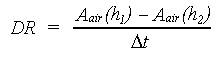
When the groundwater is within the root zone, the drainage rate is equivalent to the percolation rate. The preliminary infiltration rate (see eq. 6.26 and 6.27) cannot exceed the available soil air volume ("over saturation"). The adjusted infiltration rate is thus established by limiting the preliminary infiltration to the available soil air volume. The maximum value the adjusted infiltration rate can reach is defined as:

(6.50)

where	INmax	:	Maximum infiltration rate	[cm d-1]
	Zt	:	Depth of groundwater table at time step t	[cm]
	qair,t	:	Air content above groundwater table (see eq. 6.49)	[cm3 cm-3]
	Ta	:	Actual transpiration rate (see eq. 6.14)	[cm d-1]
	Es	:	Evaporation rate of a shaded soil surface (see eq. 6.20)	[cm d-1]
	Perc	:	Percolation rate	[cm d-1]

Two different situations are distinguished: (i)during current time step the groundwater stays within the rootzone or (ii) the groundwater level drops below the root zone. When the groundwater table stays within the root zone, the change in groundwater depth can be established with the transpiration, evaporation, percolation and infiltration rates. Transpiration, evaporation and percolation cause an increase of the air amount in the root zone, whereas the infiltration causes a decrease.

(6.50)

where	DZ	:	Change in groundwater level per time step	[cm d-1]
	IN	:	Infiltration rate	[cm d-1]
	Ta	:	Actual transpiration	[cm d-1]
	Es	:	Evaporation rate	[cm d-1]
	Perc	:	Percolation rate	[cm d-1]
	qair,t	:	Air content above groundwater table	[cm3 cm-3]

When the groundwater level falls below the root zone, water is recovered from the subsoil to maintain a stable moisture content during the transition in the rooted zone. In the water balance of the rooted zone this water amount is accounted for as capillary rise. This rather artificial construction is used because the time step of one day is too large to keep track of fluctations of the groundwater level.

(6.52)

where	CR	:	Rate of capillary rise	[cm d-1]
	DZ	:	Change in groundwater level per time step	[cm d-1]
	Zt	:	Depth of groundwater table at time step	[cm d-1]
	Dt	:	Time step	[d]
	RD	:	Actual rooting depth	[cm]
	qair,t	:	Air content above groundwater table	[cm3 cm-3]

The equilibrium profile is assumed again. The new height of the root zone above the groundwater level can now be obtained from the relation between height above the groundwater table and the cumulative air amount y(A _air), by introducing CR.Dt, the replaced air amount between the root zone and the groundwater level, into this relation. and the rate of change of the groundwater depth can be found by subtracting the old value of the groundwater depth from the new value (see eq. 6.48).
 

Moisture amount

The root zone moisture change rate is calculated in a straightforward way from the calculated flow rates:

(6.53)

where	DW	:	Rate of change in the moisture amount in the root zone	[cm d-1]
	Ta	:	Actual transpiration rate	[cm d-1]
	Es	:	Evaporation rate	[cm d-1]
	Perc	:	Percolation rate	[cm d-1]
	CR	:	Rate of capillary rise	[cm d-1]
	IN	:	Infiltration rate	[cm d-1]

 

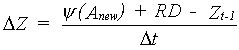
Root extension

As a result of root extension into the lower zone extra soil moisture becomes available, which can be calculated as:

(6.54)

where	DWrz	:	Change of soil moisture amount in the root zone	[cm]
	RDt	:	Rooting depth at time step t	[cm]
	Aair(h)	:	Air amount as a function of height above groundwater table (see eq. 6.39)	[cm]
	Zt	:	Depth of the groundwater table at time step t	[cm]
	qmax	:	Soil porosity	[cm3 cm-3]
	h1	:	Zt - RDt	[cm]
	h2	:	Zt-1 - RDt-1	[cm]

It is clear that the air amount in the lower zone as well as the equilibrium soil moisture amount below the rooted zone are reduced by the extension of the roots. With equation 6.54 the actual water amount in the root zone and in the lower zone can be calculated according to:

(6.55)

where	Wrz,t	:	Soil moisture amount in the root zone at time step t	[cm]
	Wrz,t-1	:	Soil moisture amount in the root zone at time step t-1	[cm]
	DWrz	:	Change of the soil moisture amount in the root zone	[cm]

 

Actual soil moisture content

The actual moisture content can now be calculated according to (see also eq. 6.1 and 6.34):

(6.56)

where	qt	:	Actual soil moisture content at time step t	[cm3 cm-3]
	Wrz,t	:	Soil moisture amount in the root zone at time step t	[cm]
	RD	:	Actual rooting depth	[cm]

The simulation stops when more than ten succesive days of waterlogging occur and the crop cannot develop airducts. Waterlogging is defined as a groundwater depth of less than 10 cm.
 
 

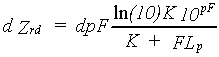
6.5. Calculation of capillary flow

Capillary flow is defined as the flow between the groundwater table and the root zone, whereas percolation is defined as the flow from the root zone to the groundwater. The flow is calculated for a stationary situation, which means that the soil moisture profile does not change within one time step. The basic equation is given by:

(6.57)

where	FLp	:	Flow rate	[cm d-1]
	Zrd	:	Distance between root zone and groundwater table	[cm]
	K	:	Hydraulic conductivity	[cm d-1]
	y	:	Matric head	[cm]

Equation 6.57 can be rewritten according to:

(6.58)

where	Zrd	:	Distance between root zone and groundwater table	[cm]
	K	:	Hydraulic conductivity	[cm d-1]
	y	:	Matric head	[cm]
	FLp	:	Flow rate	[cm d-1]

Between groundwater and rootzone a y-profile exists. An increase in Z implies an increase in y. Close to the groundwater the hydraulic conductivity is relatively large and the ratio K/(K+FL_p) is close to unity. At some height above the groundwater table the hydraulic conductivity becomes smaller and this ratio starts to decrease fast. Consequently, for a large value of y, a small increase of groundwater level will lead to large in y. A stationary soil moisture profile implies a flow rate independent of the height above the groundwater table. The hydraulic conductivity as a function of the y is known and consequently the right hand side of equation 6.58 depends only on y and can be numerically integrated over the interval (0-y_rootzone), at least, after an estimate of the flow has been made. If the resulting height difference, Z_rd, is equal to the real distance between rootzone and groundwater, D, the estimated flow is correct. If Z_rd is greater than D, however, the estimated flow is too low and if Z_rd is less than D, the estimated flow is too high. Via an iteration procedure the value of flow can be adjusted until a satisfactory value is found.
 

Initialization

The matric head can be calculated from a pF curve using:

(6.59)

where	y	:	Matric head	[cm]
	pF	:	pF value	[-]

The pF value in equation 6.59 is calculated using the AFGEN table with the soil moisture content as the independent variable (see also Subsection 6.4.2 Initialization). If the calculated matric head is smaller than or equal to zero the hydraulic conductivity is set equal to the saturated conductivity. For these conditions the flow can be calculated as:

(6.60)

where	FL	:	Flow rate	[cm d-1]
	K	:	Hydraulic conductivity	[cm d-1]
	y	:	Matric head	[cm]
	D	:	Height difference between the root zone and the groundwater table	[cm]

 

Integration

If the calculated matric head is positive, the flow rate has to be derived by means of an iteration loop. However, first the number and width of the integration intervals has to be established. The maximum number of integration intervals equals four, their width's are defined as: [0-45 cm], [45-170 cm], [170-330 cm] and [330,y_rootzone].
To integrate the last interval, a logarithmic transformation is applied. This interval is then written as (¹⁰log(330), ¹⁰log(y_rootzone)).
If for example the matric head is 220 cm, only three integration intervals will be included: [0-45 cm], [45-170 cm], [170-220 cm]. If the matric head is larger than 330 cm a fourth integration interval will be included. The width of the fourth interval will than be calculated as pF minus ¹⁰log330. Using a logarithmic transformation, equation 6.55 becomes:

(6.61)

where	Zrd	:	Distance between root zone and groundwater table	[cm]
	K	:	Hydraulic conductivity	[cm d-1]
	pF	:	pF value	[-]
	FLp	:	Flow rate	[cm d-1]

The three point Gaussian integration is used for the integration of y over the intervals mentioned above. The length of each integration interval can be expressed as:

(6.62)

where	Dy	:	Length of the interval matric head	[cm]
	y0	:	Lower boundary interval matric head	[cm]
	y1	:	Upper boundary interval matric head	[cm]

According to the Gaussian integration method, three distances within the length of the integration interval are selected:

for

p= -1,0,1

(6.63)

where	yi	:	Matric head	[cm]
	p	:	Three points of the Gaussian integration

The selected matric head values for Gaussian integration for each integration interval can be calculated as:

(6.64)

where	y	:	Total selected matric head	[cm]
	y0	:	Lower boundary interval matric head	[cm]
	Dyi	:	Selected matric head	[cm]

The selected matric head values can be expressed as pF-values according:

(6.65)

where	pF	:	pF-value	[-]
	y	:	Matric head	[cm]

For the full-width integration intervals, the selected matric head values and therefore the selected pF-values will always be the same. With the equations 6.62, 6.63 and 6.64, the three selected matric heads per interval for the Gaussian integration can be calculated. With the help of equation 6.65, the pF-values for the full-width integration intervals can be calculated. The results are presented in Table 6.3.
 

Table 6.3. pF values of the selected matric heads per interval.

pF-values
[0, 45]	0.705143	1.352183	1.601282
[45, 170]	1.771497	2.031409	2.192880
[170, 330]	2.274233	2.397940	2.494110

 

To diminish calculation time the pF-values for the full width integration intervals should be included. For different integration intervals the calculations are the same. For the last interval, as mentioned before, a logarithmic transformation is applied. Instead of matric head values, now three pF values are selected, using the Gaussian integration method.

for

p= -1,0,1

(6.66)

where	pFi	:	pF value	[-]
	p	:	Three points of the Gaussian integration

As mentioned earlier, first the intervals have to be selected. For these intervals, for every selected hydraulic head or pF-value three per interval), the hydraulic conductivity is computed using the following equation:

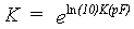(6.67)

where	K	:	Hydraulic conductivity	[cm d-1]
	K(pF)	:	10log of hydraulic conductivity as a function of pF	[-]

The ¹⁰log of hydraulic conductivity as a function of pF, K(pF), is soil specific and should be provided by the user. The values of K, calculated with equation 6.67, are needed in the iteration loop to calculate (K+FL_p), the denominator of equation 6.58. The nominator of the right-hand side of equation 6.58 is integrated using the Gaussian integration. Therefore, the K values are multiplied by the size of the interval (DY) and by the weighing factor. The results are put in a help array.
 

Iteration

In order to find the correct flow rate in the iteration process, an upper limit and a lower limit have to be established. The actual flow rate lies somewhere in between. The upper limit of the flow rate is set to 1.27 cm d^-1 and lower limit for the flow rate can be set as:

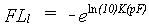(6.68)

where	FLl	:	Lower limit for the flow rate	[cm d-1]
	K(pF)	:	Hydraulic conductivity as a function of the pF	[-]

The estimated flow rate is chosen halfway between the upper and lower limit. After the flow rate estimation, the iteration process starts. The calculated height above the groundwater table is compared with the real distance between root zone and groundwater. Depending on the outcome, either the upper limit or the lower limit is adjusted, and the process starts again. If the absolute error is smaller then 0.01 and the relative error smaller than 0.1, the iteration is terminated. The iteration is limited to a maximum of 15 steps.

It is assumed that the rate of capillary rise is never higher than 1.27 cm d^-1. If the matric head is smaller than the depth of the groundwater level, the upper limit for the flow rate is set to zero. If the matric head is larger than the groundwater depth the lower limit is set to zero. If the matric head is equal to the depth of the groundwater both, upper and lower limit are set to zero and therefore the flow rate equals zero.